|
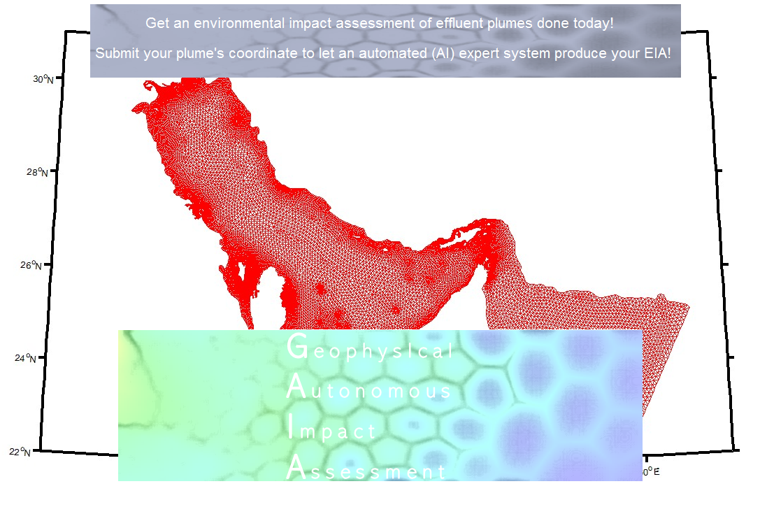
Aquifer modeling Aquifer modeling consists commonly of three differential systems. 3D SMART depicts these (and marine domains) with advanced Voronoi meshes. 1. the groundwater level simulation. The groundwater level, the water table, or, measured downwards from the surface, the groundwater head, is governed by the hydraulic pressure. Inertia, advection and turbulence play no role. That yields a very simple diffusion/conduction type partial differential equation that determines the ceiling of the water saturation of the ground. The coefficients in this system merely depend on the conductivity (here: hydraulic conductivity) and the specific storage of the ground material. Source and sink terms, depending on conducted water injection or removal respectively, alter the initial groundwater head distribution. 2. Proportional to the gradient of the groundwater level is the fluid flux. Henceforth, the flow field can be readily obtained by simulating the trivial conductivity PDE from # 1. 3. The pollutant or contaminant fate simulation in turn is driven by the flow field obtained in step # 2. A common task for characterising a diffusive PDE are in general and in aquifer modeling as well parameter identification iterations. That is, the simulation is repeated with different coefficients to fit results to measurements. The 3D Shelf Marine and Atmosphere Reactive Transport (3D SMART) model harnesses besides the marine and atmosphere domain also the shelf ground domain. Results of computer fluid dynamic simulations are then run through the symbolic, or rule based, AI to ID compliance and, if any, impact. That is, http://www.wavedyne.com is rapidly converging to offering you far superior and near instantaneous environmental impact assessments.
Contact: info@environment.report |
